Walker Alloy 617 model subsystem

This subsystem implements the constitutive model described by Sham and Walker [SW2008], aimed at capturing the long-term response of Alloy 617. The subsystem also prototypes merging the History object system system for maintaining named and tagged internal history variables with the base constitutive model system using flat vectors.

The subsystem contains Viscoplastic flow rule, Hardening models, and several dedicated submodels representing special functions in Walker’s model. This document provides a description of the entire subsystem. Later, the history-wrapped models will replace the current flat vector system and this documentation can be merged into the main NEML module documentation.

Mathematical description

This description is extracted from an Argonne National Laboratory technical report describing the implementation of the model [MS2020].

Basic viscoplastic response

The model starts with the basic inelastic stress rate equation:

$\dot{\bm{\sigma}}=\boldsymbol{C}:\left(\dot{\bm{\varepsilon}}-\dot{\bm{\varepsilon}}_{vp}-\dot{\bm{\varepsilon}}_{th}\right)$

with $\dot{\bm{\sigma}}$ the stress rate, $\boldsymbol{C}$ an isotropic elasticity tensors described by Young’s modulus $E$ and Poisson’s ratio $\nu$ , $\dot{\bm{\varepsilon}}$ the total (applied) strain rate, $\dot{\bm{\varepsilon}}_{vp}$ is the viscoplastic strain rate described below, and $\dot{\bm{\varepsilon}}_{th}$ is the thermal strain rate given by

$\dot{\bm{\varepsilon}}_{th}=\alpha\dot{T}\boldsymbol{I}$

with $\alpha$ the instantaneous coefficient of thermal expansion, $\dot{T}$ the temperature rate, and $\boldsymbol{I}$ the identity tensor.

The model definition reuses several common functions. These functions appear several places in the formulation, occasionally with the same parameters and occasionally with different parameters depending on the location. Where needed this exposition distinguishes the function parameters using parenthetical superscripts, e.g. $x^{\left(a\right)}$ .

Temperature scaling function

The temperature scaling function:

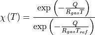
$\chi\left(T\right)=\frac{\exp\left(-\frac{Q}{R_{gas}T}\right)}{\exp\left(-\frac{Q}{R_{gas}T_{ref}}\right)}$

with $Q$ an activation energy, $R_{gas}$ the gas constant, and $T_{ref}$ a reference temperature, with temperature in Kelvin, is reused several places in the model. The thermal scaling constants $Q$ and $T_{ref}$ remain the same with each appearance and so no superscripts are required.

Strain softening/tertiary creep function

The tertiary creep function

$\Phi=1+\phi_{0}p^{\phi_{1}}$

with $p$ the equivalent plastic strain and $\phi_{0}$ and $\phi_{1}$ temperature-dependent constants likewise appears several times in the model. Different components of the model uses different parameters $\phi_{0}$ and $\phi_{1}$ , differentiated by superscripts.

The viscoplastic strain rate

The viscoplastic strain rate is

$\dot{\bm{\varepsilon}}_{vp}=\dot{p}\boldsymbol{g}$

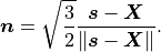
where $\dot{p}$ is the scalar plastic strain rate and $\boldsymbol{g}$ the flow direction. The flow direction is

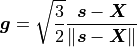
$\boldsymbol{g}=\sqrt{\frac{3}{2}}\frac{\boldsymbol{s}-\boldsymbol{X}}{\left\Vert \boldsymbol{s}-\boldsymbol{X}\right\Vert }$

with $\boldsymbol{s}$ the deviatoric part of the stress, $\bm{s}=\operatorname{dev}\left(\bm{\sigma}\right)$ and $\boldsymbol{X}$ the backstress defined below. In this expression and in the equations below the tensor norm is defined as

$\left\Vert \boldsymbol{Y}\right\Vert =\sqrt{\boldsymbol{Y}:\boldsymbol{Y}}$

with $:$ indicating double contraction.

The scalar strain rate is

$\dot{p}=\dot{\varepsilon}_{0}\Phi^{\left(p\right)}\left(p\right)\chi\left(T\right)F\label{eq:plastic-rate}$

with $\dot{\varepsilon}_{0}$ , $\Phi^{\left(p\right)}\left(p\right)$ a softening function defined by constants $\phi_{0}^{\left(p\right)}$ and $\phi_{1}^{\left(p\right)}$ , $\chi\left(T\right)$ the temperature scaling function, and $F$ the flow function

$F=\left\langle \frac{\sqrt{3/2}\left\Vert \boldsymbol{s}-\boldsymbol{X}\right\Vert -Y}{D}\right\rangle ^{n}$

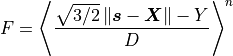
with $D$ an internal variable defined later, $n$ a parameter, $\left\langle \right\rangle$ the Macaulay brackets, and $Y$ the threshold stress given as

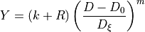
$Y=\left(k+R\right)\left(\frac{D-D_{0}}{D_{\xi}}\right)^{m}$

with $k$ , $D_{0}$ , $D_{\xi}$ , and $m$ parameters and $R$ an internal variable defined below.

Isotropic hardening

The isotropic hardening variable evolves as

$\dot{R}=r_{0}\left(R_{\infty}-R\right)\dot{p}+r_{1}\left(R_{0}-R\right)\left|R_{0}-R\right|^{r_{2}-1}\label{eq:R}$

where $r_{0}$ , $R_{\infty}$ , $r_{1}$ , $R_{0}$ , and $r_{2}$ are all parameters. The initial value of the isotropic hardening parameter is zero.

Kinematic hardening

The net backstress is the sum of three individual backstress terms:

$\boldsymbol{X}=\sum_{i=1}^{3}\boldsymbol{X}_{i}. The evolution equation for each individual backstress is$

$\dot{\boldsymbol{X}}=\frac{2}{3}c\left(p,\dot{p}\right)\dot{\bm{\varepsilon}}_{vp}-\frac{c\left(p,\dot{p}_{0}\right)}{L\left(p\right)}\dot{p}\boldsymbol{b}-\chi\left(T\right)x_{0}\Phi^{\left(x\right)}\left(p\right)\left(\sqrt{\frac{3}{2}}\frac{\left\Vert \boldsymbol{X}\right\Vert }{D}\right)^{x_{1}}\frac{\boldsymbol{X}}{\left\Vert \boldsymbol{X}\right\Vert }\label{eq:X}$

where $x_{0}$ and $x_{1}$ are parameters, $c\left(p,\dot{p}\right)$ , is a function defined below of the the equivalent plastic strain, $p$ and either the actual plastic strain $\dot{p}$ or a reference plastic strain rate $\dot{p}_{0}$ , $\Phi^{\left(x\right)}\left(p\right)$ is a softening function with independent parameters,

$L\left(p\right)=l\left(l_{1}+\left(1-l_{1}\right)\exp\left[-l_{0}p\right]\right)$

with $l$ , $l_{0}$ , and $l_{1}$ parameter, and

$\boldsymbol{b}=\left(1-b_{0}\right)\boldsymbol{X}+\frac{2}{3}b_{0}\left(\boldsymbol{n}\otimes\boldsymbol{n}\right):\boldsymbol{X}$

with $b_{0}$ a parameter and

$\boldsymbol{n}=\sqrt{\frac{3}{2}}\frac{\boldsymbol{s}-\boldsymbol{X}}{\left\Vert \boldsymbol{s}-\boldsymbol{X}\right\Vert }.$

In these expressions the outer product symbol $\otimes$ between two rank two tensors denotes the product given in index notation as

$\boldsymbol{a}\otimes\boldsymbol{b}=a_{ij}b_{kl}.$

The backstresses all start at $\boldsymbol{X}=\boldsymbol{0}$ .

Walker’s original model defined

$c\left(p,\dot{p}\right)=\left\{ c_{0}+c_{1}\dot{p}^{1/c_{2}}\right\} \Omega\left(p\right)$

with the $\Omega$ function of the equivalent plastic strain given as

$\Omega\left(p\right)=1+\left(\frac{D-D_{0}}{D_{\xi}}\right)^{\omega_{0}}\omega\left(p\right)\left(\omega_{1}-1\right)\exp\left(-\omega_{2}q\right)$

with $\omega_{0}$ , $\omega_{1}$ , and $\omega_{2}$ parameters. The function $\omega\left(p\right)$ is defined as

$\omega\left(p\right)=\omega_{3}+\left(1-\omega_{3}\right)\exp\left[-\omega_{4}p\right]$

with $\omega_{3}$ and $\omega_{4}$ additional parameters and $q$ is an additional internal variable with evolution equation

$\dot{q}=\dot{p}-\chi\left(T\right)q_{0}q$

where $q_{0}$ is a parameter and $q\left(0\right)=0$ . The function $\Omega\left(p\right)$ and the associated internal variable describe the stress overshoot in the cyclic tests

This implementation omits the overshoot part of the model, leaving

$c\left(\dot{p}\right)=c_{0}+c_{1}\dot{p}^{1/c_{2}}$

with $c_{0}$ , $c_{1}$ , and $c_{2}$ parameters. Depending on the location of the $c$ function (in the hardening or dynamic recovery terms), this function is either invoked with the actual plastic strain rate $\dot{p}$ or with some constant rate $\dot{p}_{0}$ , which is a model parameter.

The subsequent tables differentiate the parameters for each backstress using superscripted indices.

Drag stress evolution

The drag stress evolves as

$\dot{D}=d_{0}\left(1-\frac{D-D_{0}}{D_{\xi}}\right)\dot{p}-\chi\left(T\right)\Phi^{\left(D\right)}\left(p\right)d_{1}\left(D-D_{0}\right)^{d_{2}}\label{eq:D}$

where $d_{0}$ , $D_{\xi}$ , $d_{1}$ , and $d_{2}$ are parameters, and $\Phi^{\left(D\right)}\left(p\right)$ is a softening function with independent coefficients.

NEML implementation

The implementation includes a wrapper for the full history subsystem and the implementation within the wrapper of the walker flow rule and a simple test flow rule, for debugging the wrapper functions.

The model implements the various subcomponents of the flow rule as individual classes